Standardization involves transforming dataset with Gaussian distribution to 0 mean and unit variance (standard deviation of 1).
Many learning algorithms assume that all features are centered around 0 and have variance in the same order
This recipe includes the following topics:
- Standarize using StandardScaler class
- Call fit() to compute the mean and std to be used for later scaling
- Call transform() on the input data
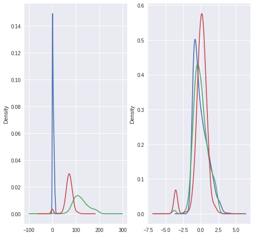
- Draw KDE plots to compare before and after Standardization
# import modules
import pandas as pd
import numpy as np
import matplotlib.pyplot as plt
from sklearn.preprocessing import StandardScaler

# read data file from github
# dataframe: pimaDf
gitFileURL = 'https://raw.githubusercontent.com/andrewgurung/data-repository/master/pima-indians-diabetes.data.csv'
cols = ['preg', 'plas', 'pres', 'skin', 'test', 'mass', 'pedi', 'age', 'class']
pimaDf = pd.read_csv(gitFileURL, names = cols)

# convert into numpy array
pimaArr = pimaDf.values

# Though we won't be using the test set in this example
# Let's split our data into the usual train(X) and test(Y) set
X = pimaArr[:, 0:8]
Y = pimaArr[:, 8]

# 1. initiate StandardScaler class
# 2. call fit() to compute the mean and std
scaler = StandardScaler().fit(X)

# standarize input data using transform()
rescaledX = scaler.transform(X)

# limit precision to 3 decimal points for printing
np.set_printoptions(3)

# print first 3 rows of input data
print(X[:3,])
print('-'*60)

# print first 3 rows of output data
print(rescaledX[:3,])

# draw kde plot to see the transformation visually
# add two subplots
fig, (ax1, ax2) = plt.subplots(ncols=2, figsize=(8, 8))

# plot KDE for input data
pimaDf['preg'].plot.kde(ax=ax1)
pimaDf['plas'].plot.kde(ax=ax1)
pimaDf['pres'].plot.kde(ax=ax1)


# convert rescaledX array to DataFrame
rescaledDf = pd.DataFrame(rescaledX, columns=['preg', 'plas', 'pres', 'skin', 'test', 'mass', 'pedi', 'age'])

# plot KDE for input data
rescaledDf['preg'].plot.kde(ax=ax2)
rescaledDf['plas'].plot.kde(ax=ax2)
rescaledDf['pres'].plot.kde(ax=ax2)
plt.show()of output data
print(rescaledX[:3,])
[[  6.    148.     72.     35.      0.     33.6     0.627  50.   ]
 [  1.     85.     66.     29.      0.     26.6     0.351  31.   ]
 [  8.    183.     64.      0.      0.     23.3     0.672  32.   ]]
------------------------------------------------------------
[[ 0.64   0.848  0.15   0.907 -0.693  0.204  0.468  1.426]
 [-0.845 -1.123 -0.161  0.531 -0.693 -0.684 -0.365 -0.191]
 [ 1.234  1.944 -0.264 -1.288 -0.693 -1.103  0.604 -0.106]]